Sorting Algorithms
![]()
The common sorting algorithms can be divided into two classes by the complexity of their algorithms. Algorithmic complexity is a complex subject (imagine that!) that would take too much time to explain here, but suffice it to say that there's a direct correlation between the complexity of an algorithm and its relative efficiency. Algorithmic complexity is generally written in a form known as Big-O notation, where the O represents the complexity of the algorithm and a value n represents the size of the set the algorithm is run against.
The O(n) means that an algorithm has a linear complexity. In other words, it takes ten times longer to operate on a set of 100 items than it does on a set of 10 items (10 * 10 = 100). If the complexity was O(n2) (quadratic complexity), then it would take 100 times longer to operate on a set of 100 items than it does on a set of 10 items.
The two classes of sorting algorithms are O(n2), which includes the bubble, insertion, selection, and shell sorts; and O(n log n) which includes the heap, merge, and quick sorts.
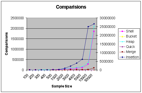
In addition to algorithmic complexity, the speed of the various sorts can be compared with diffrent type of data. Since the speed of a sort can vary greatly depending on what data set it sorts, accurate empirical results require several runs of the sort be made and the results averaged together.
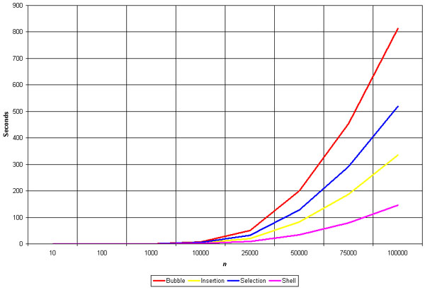
As the graph pretty plainly shows, the bubble sort is grossly inefficient, and the shell is the fastest.
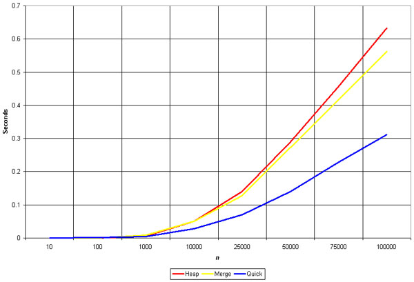
The O(n log n) sorts are the fastest. These algorithms are blazingly fast, but that speed comes at the cost of complexity. Recursion, advanced data structures, multiple arrays.
Insertion Sort
![]()
Algorithm
Analysis
The insertion sort works just like its name suggests - it
inserts each item into its proper place in the final list. The simplest
implementation of this requires two list structures - the source list and the
list into which sorted items are inserted. To save memory, most implementations
use an in-place sort that works by moving the current item past the already
sorted items and repeatedly swapping it with the preceding item until it is in
place.
Like the bubble sort, the insertion sort has a complexity of O(n2). Although it has the same complexity, the insertion sort is a little over twice as efficient as the bubble sort.
Pros: Relatively simple and easy to
implement.
Cons: Inefficient for large lists.
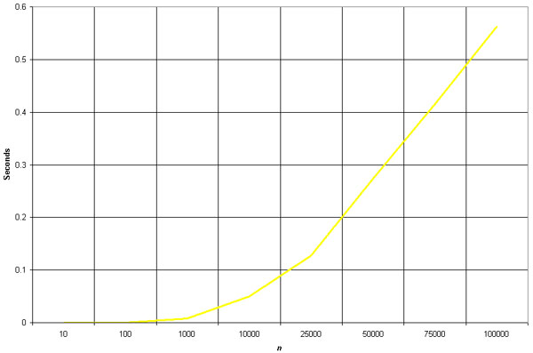
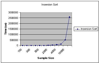
Empirical Analysis

The graph demonstrates the n2 complexity of the insertion sort.
The insertion sort is a good middle-of-the-road choice for sorting lists of a few thousand items or less. The algorithm is significantly simpler than the shell sort, with only a small trade-off in efficiency. At the same time, the insertion sort is over twice as fast as the bubble sort and almost 40% faster than the selection sort. The insertion sort shouldn't be used for sorting lists larger than a couple thousand items or repetitive sorting of lists larger than a couple hundred items.
Shell Sort
![]()
Algorithm Analysis
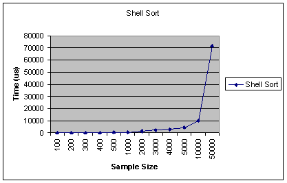
Invented by Donald Shell in 1959, the shell sort is the most efficient of the O(n2) class of sorting algorithms. Of course, the shell sort is also the most complex of the O(n2) algorithms.
The shell sort is a "diminishing increment sort", better known as a "comb sort" to the unwashed programming masses. The algorithm makes multiple passes through the list, and each time sorts a number of equally sized sets using the insertion sort. The size of the set to be sorted gets larger with each pass through the list, until the set consists of the entire list. (Note that as the size of the set increases, the number of sets to be sorted decreases.) This sets the insertion sort up for an almost-best case run each iteration with a complexity that approaches O(n).
The items contained in each set are not contiguous - rather, if there are i sets then a set is composed of every i-th element. For example, if there are 3 sets then the first set would contain the elements located at positions 1, 4, 7 and so on. The second set would contain the elements located at positions 2, 5, 8, and so on; while the third set would contain the items located at positions 3, 6, 9, and so on.
The size of the sets used for each iteration has a major impact on the efficiency of the sort. Several Heroes Of Computer ScienceTM, including Donald Knuth and Robert Sedgewick, have come up with more complicated versions of the shell sort that improve efficiency by carefully calculating the best sized sets to use for a given list.
Pros: Efficient for medium-size lists.
Cons:
Somewhat complex algorithm, not nearly as efficient as the merge, heap, and quick sorts.
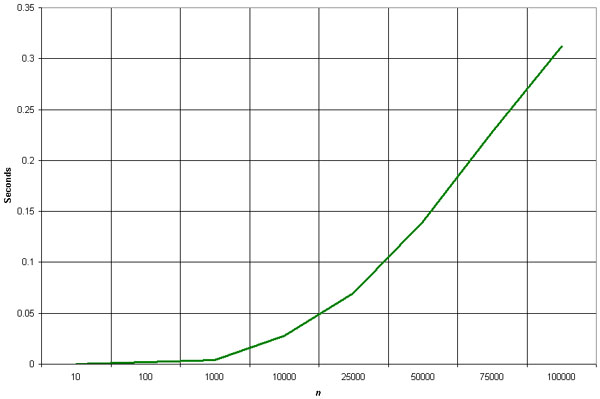
Empirical Analysis
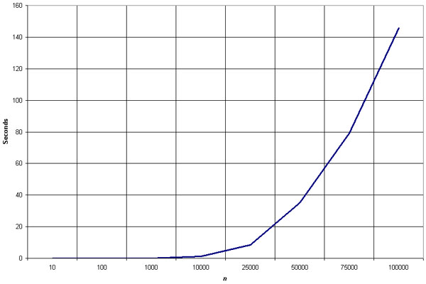
The shell sort is by far the fastest of the N2 class of sorting algorithms. It's more than 5 times faster than the bubble sort and a little over twice as fast as the insertion sort, its closest competitor.
The shell sort is still significantly slower than the merge, heap, and quick sorts, but its relatively simple algorithm makes it a good choice for sorting lists of less than 5000 items unless speed is hyper-critical. It's also an excellent choice for repetitive sorting of smaller lists.
Heap Sort
![]()
Algorithm Analysis
The heap sort is the slowest of the O(n log n) sorting algorithms, but unlike the merge and quick sorts it doesn't require massive recursion or multiple arrays to work. This makes it the most attractive option for very large data sets of millions of items.
The heap sort works as it name suggests - it begins by building a heap out of the data set, and then removing the largest item and placing it at the end of the sorted array. After removing the largest item, it reconstructs the heap and removes the largest remaining item and places it in the next open position from the end of the sorted array. This is repeated until there are no items left in the heap and the sorted array is full. Elementary implementations require two arrays - one to hold the heap and the other to hold the sorted elements.
To do an in-place sort and save the space the second array would require, the algorithm below "cheats" by using the same array to store both the heap and the sorted array. Whenever an item is removed from the heap, it frees up a space at the end of the array that the removed item can be placed in.
Pros: In-place and non-recursive, making it a good
choice for extremely large data sets.
Cons: Slower than the merge and quick sorts.
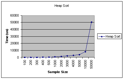
Empirical Analysis
As mentioned above, the heap sort is slower than the merge and quick sorts but doesn't use multiple arrays or massive recursion like they do. This makes it a good choice for really large sets, but most modern computers have enough memory and processing power to handle the faster sorts unless over a million items are being sorted.
The "million item rule" is just a rule of thumb for common applications - high-end servers and workstations can probably safely handle sorting tens of millions of items with the quick or merge sorts. But if you're working on a common user-level application, there's always going to be some yahoo who tries to run it on junk machine older than the programmer who wrote it, so better safe than sorry.
![]()
Quick Sort
![]()
Algorithm Analysis
The quick sort is an in-place, divide-and-conquer, massively recursive sort. As a normal person would say, it's essentially a faster in-place version of the merge sort. The quick sort algorithm is simple in theory, but very difficult to put into code (computer scientists tied themselves into knots for years trying to write a practical implementation of the algorithm, and it still has that effect on university students).
The recursive algorithm consists of four steps (which closely resemble the merge sort):
The efficiency of the algorithm is majorly impacted by which element is choosen as the pivot point. The worst-case efficiency of the quick sort, O(n2), occurs when the list is sorted and the left-most element is chosen. Randomly choosing a pivot point rather than using the left-most element is recommended if the data to be sorted isn't random. As long as the pivot point is chosen randomly, the quick sort has an algorithmic complexity of O(n log n).
Pros: Extremely fast.
Cons: Very complex
algorithm, massively recursive.
PRESENTATION OF THE QUICK SORT
The quick sort is an in-place, divide-and-conquer, massively recursive sort. It consists in 4 steps :
| If there are one or less elements in the array to be sorted, return immediately | |
| Pick an element in the array to serve as a "pivot" point. Here, we chose the left-most item. | |
| Split the array into 2 parts : the left one with elements smaller than the pivot and the right with elements larger. | |
| Recursively repeat the algorithm for both halves of the original array. |
For example, we took the same array as for the bubble sort :
|
Element
|
1 |
2 |
3 |
4 |
5 |
6 |
7 |
8 |
|
Data |
14 |
27 |
8 |
89 |
6 |
12 |
36 |
19 |
|
1st pass
|
12
|
6
|
8
|
14
|
89 |
27 |
36 |
19 |
|
2nd pass
|
8 |
6 |
12 |
14 |
89 |
27 |
36 |
19 |
|
3rd pass
|
6
|
8 |
12 |
14 |
89 |
27 |
36 |
19 |
|
4th pass
|
6 |
8 |
12 |
14 |
19
|
27
|
36
|
89 |
|
5th pass |
6 |
8 |
12 |
14 |
19 |
27 |
36 |
89 |
|
6th pass |
6 |
8 |
12 |
14 |
19 |
27 |
36 |
89 Sorted ! |
Number in red : the pivot
Numbers in blue : left sub-list Numbers in green : right sub-list
Numbers in italic : items no sorted (in the current pass) Numbers in black : sorted items
The quick sort takes the first element :14, and places it such that all the numbers in the left sub-list are smaller and all the numbers in the right sub-list are bigger. It then quick sorts the left sub-list : {12,6,8} and then quick sorts the right sub-list {89,27,36,19}.
Passes 2 and 3 : quicksort for the items on the left of 14.
Passes 4, 5 and 6 : quicksort for the items on the right of 14. We can notice that in this example, the array is already in the 4th pass, but the algorithm continues until there isn't test to make any more.
This is a recursive algorithm, since it is defined in terms of itself. This reduces the complexity of programming it, however it is one of the least intuitive algorithm.
Worst Case
The worst case occurs when
in each recursion step an unbalanced partitionning is produced, namely that one
part consists of only one element and the other part consists of the rest of the
elements. A such case is encountered when the array is already ordered or in
reverse order. Then the recursion depth is n-1 and the complexity of
quicksort in (n2).
We define CN as the cost of sorting N elements
:
 |
 |
 |
|
|
 |
||
|
 |
||
|
 |
||
 |
|||
|
 |
||
|
 |
||
|
 |
||
|
 |
The best-case behavior of the Quicksort
algorithm occurs when in each recursion step the partitionning produces two
parts of equal length. So at each time, the pivot must be the median of the
values. In order to sort n elements, in this case the complexity and the running
time are in (nlog2(n)). This is because
the recursion depth is log(n) and on each level there are n elements to be
treated.
We define CN as the cost of sorting N elements :
Supposed(
is the cost of the
elements)
 :
:

 |
|
 |
|
|
 |
||
|
|||
|
 |
||
|
 |
|
|
(1) | ||
|
|
(2) |

Empirical Analysis
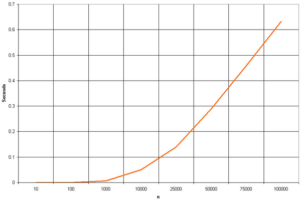
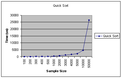
The quick sort is by far the fastest of the common sorting algorithms. It's possible to write a special-purpose sorting algorithm that can beat the quick sort for some data sets, but for general-case sorting there isn't anything faster.
As soon as students figure this out, their immediate implulse is to use the quick sort for everything - after all, faster is better, right? It's important to resist this urge - the quick sort isn't always the best choice. As mentioned earlier, it's massively recursive (which means that for very large sorts, you can run the system out of stack space pretty easily). It's also a complex algorithm - a little too complex to make it practical for a one-time sort of 25 items, for example.
With that said, in most cases the quick sort is the best choice if speed is important (and it almost always is). Use it for repetitive sorting, sorting of medium to large lists, and as a default choice when you're not really sure which sorting algorithm to use. Ironically, the quick sort has horrible efficiency when operating on lists that are mostly sorted in either forward or reverse order - avoid it in those situations.
![]()
Merge Sort
![]()
Algorithm Analysis
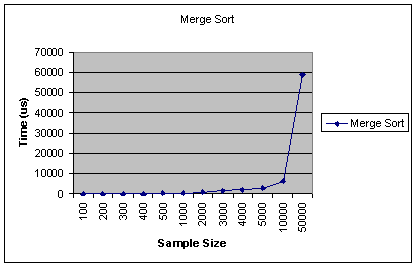
The merge sort splits the list to be sorted into two equal halves, and places them in separate arrays. Each array is recursively sorted, and then merged back together to form the final sorted list. Like most recursive sorts, the merge sort has an algorithmic complexity of O(n log n).
Elementary implementations of the merge sort make use of three arrays - one for each half of the data set and one to store the sorted list in. The below algorithm merges the arrays in-place, so only two arrays are required. There are non-recursive versions of the merge sort, but they don't yield any significant performance enhancement over the recursive algorithm on most machines.
Pros: Marginally faster than the heap sort for larger
sets.
Cons: At least twice the memory requirements of the other sorts;
recursive.
Empirical Analysis
The merge sort is slightly faster than the heap sort for larger sets, but it requires twice the memory of the heap sort because of the second array. This additional memory requirement makes it unattractive for most purposes - the quick sort is a better choice most of the time and the heap sort is a better choice for very large sets.
Like the quick sort, the merge sort is recursive which can make it a bad choice for applications that run on machines with limited memory.
![]()
Run Data
![]()
The run of the program is saved as a text file 'output.txt' which is attached in the tar.
Final Run Time Graphs
![]()
Complexity Graphs
![]()
Comparison Hybrid - Quick Sort
![]()
![]()

